Near Vertical Incident Skywave (NVIS) Antennas

last updated 28 November 2023.

New to NVIS? Here is a Beginner’s Guide to NVIS to get you started.

Hams have been making local contacts on 80m and 40m long before this mode was given such a fancy name to sell it to the military in the 1960s. But as part of that process we also have more complete studies on how to optimize antennas for this purpose.

Propagation

NVIS isn’t just about antennas: it is a communications system that permits coverage up to 500 km (300 miles) or so using relatively low power equipment. To do so, the operating channels must be below the Critical Frequency, the highest frequency where signals radiated straight up will be returned to Earth by the ionosphere. Above that frequency, signals pass off into space, even though they may be reflected back when striking the ionosphere at flatter angles. Generally the critical frequency may get as high as 12 MHz in the tropics or 9 MHz at higher latitudes, depending on the current ionospheric conditions, so 160m, 80m, and 40m (and 60m where it is available) are the most likely bands to use. It varies throughout the day, with the seasons, and with the 11-year sunspot cycle, as well as with latitude. Some hams are used to thinking “40m during the day, 80m at night”, but here at 45 degrees North latitude we have needed to use 80m during the day and 160m at night more often due to poor conditions (even in summer). And when the Critical Frequency drops below 2 MHz, even 160m may not work for NVIS (although ground wave might get through).

At the other end of the spectrum, the minimum frequency is generally determined by RF absorption in the D layer, which increases with ionization. Unlike the maximum frequency, increasing power may allow sufficient signals in marginal conditions. When D layer absorption is excessive at the Critical Frequency, then NVIS won’t work.

Successful NVIS operation requires being able to change frequency to suit current conditions, rather than making assumptions and hoping the ionosphere will cooperate.

Propagation Forecasts

Fortunately, we have tools available to help choose a suitable band, like the Critical Frequency map. Click here for current critical frequency map. (Opens in a new tab.)

I find the Local Area Mobile Prediction (LAMP) forecast from the Australian Space Weather Services to be handy for planning NVIS frequencies. It shows the expected best band vs. time of day for communicating over distances out to 1000 km (600 miles). To run it, click the link above, click HF Prediction, and choose LAMP. Then click on your location on the map (or enter the data in the “Base” tab), choose your frequencies (the amateur bands presets are along the bottom buttons), select an appropriate T index, and hit PREDICT. My current plot as I am typing this looks like this:

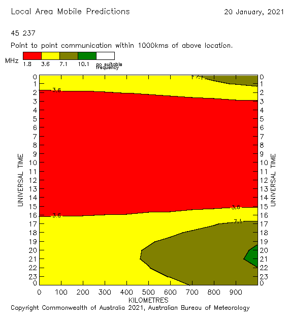
*Figure 1. Local Area Mobile Prediction forecast.*

This is run for a specific latitude, longitude, and date, based on the current conditions. The vertical axis is time of day (UTC). The horizontal axis is distance in km. Looking at the color key at the top (which will vary depending on conditions and the bands selected), for this plot the red area shows the times and distances where 160m is the best (and likely the only) band that will provide NVIS coverage. The yellow portion shows where 80m will work best. The dark olive portion shows that 40m will only be better than 80m for distances over 500 km (300 miles), and only in the middle of the day. The green spot in the lower right corner shows that 30m would open for 1000km (600 mile) paths around noon local time. Obviously, this is not a good time to expect to use 40m! (We are in winter at the bottom of the sunspot cycle, so this is not a big surprise.)

Another useful online propagation tool is VOACAP. This allows the user to specify the receiver and transmitter locations, power levels, antennas, mode, and the noise level at the receiver, then plots the probability of the path being open vs. time of day for each band. This is particularly useful for evaluating the difference in coverage with changes in antennas and power levels. Note, however, that VOACAP only covers HF, so it doesn’t include 160m, and some users have reported that it is overly optimistic at short distances.

To use it, enter the power level and mode, then drag the transmitter and receiver icons to the desired locations on the map (or enter the location data). For NVIS forecasts, you will usually want to expand the map to show more detail close to the transmitter. You can set the antenna types, then choose “Prop Charts” or “Prop Wheel” for two different ways of displaying the data.

The two programs use different algorithms, and apply different criteria for the result. The Australian forecasts are for the FOT (optimum traffic frequency), where the band will be open reliably. VOACAP calculates the probability of each band being open, rather than just the best band, and tends to show bands open more often. I suggest you try both and see which works best for your particular paths. (Both can be used for non-NVIS paths as well.)

Antenna Selection

To use NVIS, in addition to choosing an appropriate frequency where the ionosphere is cooperative, we want to radiate our signal straight up (or close to it). One advantage with this approach is that mountains between the two stations don’t obstruct the path.

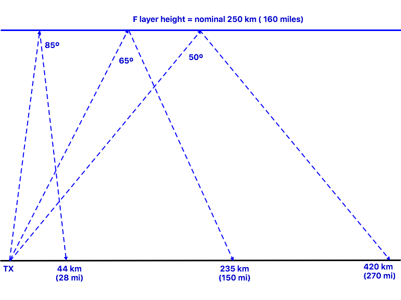
*Figure 2A. Traditional model of Distance vs. elevation angle (degrees) for an F-layer height of 250 km (160 miles)*

The required elevation angle depends on the desired distance (and the height of the ionosphere). In the drawing above, for a nominal F-layer height, signals at 85 degrees above the horizon (5 degrees from vertical) will reflect back to Earth at a distance of about 44 km (28 miles), while those at 50 degrees above the horizon (40 degrees from vertical) cover about 420km ( 270 miles).

But the ionosphere isn’t that simple. First, the effective F-layer height varies with frequency (as well as the ionospheric conditions). So the required angle to cover a specific distance (or the distance covered by a a particular vertical angle) isn’t necessarily the same for different bands. While some books show 400 km (250 miles) as a typical value, this probably is for higher frequencies used over longer distances. On the bands where NVIS is useful, a height of 200-250 km (125-160 miles) may be more typical, but it will still vary.

More importantly, as one goes lower in frequency, reflections may be off of the E-layer rather than the F-layer, which lowers the required angle to cover a distance (or reduces the distance covered by a particular vertical angle).

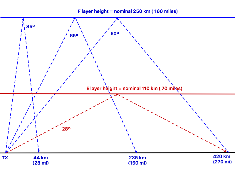
*Figure 2B. Sometimes propagation is via the E-layer instead of the F-layer*

Here we see an example where the radiation at angle of 50 degrees is reflected by the E-layer, rather than the F-layer. Now to cover 420 km (270 mi) it requires a vertical angle of 28 degrees instead of 50 degrees. The transition frequency where the E-layer becomes significant over these distances is typically between about 3.0 and 6.0 MHz, and varies with ionospheric conditions (among other factors). On 80m, this begins to have an impact somewhere between 150 and 250 km (95 to 160 mi), and it isn’t uncommon for signals near 3.5 MHz to reflect via the E-layer while those near 4.0 MHz travel via the F-layer. In most cases out to perhaps 500 km (300 miles), 40m signals will use the F-layer, while 160m signals reflect from the E-layer at almost any distance, so will require lower angles of radiation (which may be while vertical polarization works well on 160m).

For antenna planning, this means that, especially on 80m, antennas may need to be able to cover a range of vertical angles to maintain effective communications over a specific path. Any any chart or table showing a specific vertical angle vs. path length, especially if no frequency and/or ionospheric conditions are specified, is likely to be wrong much of the time, simply because such path conditions are not constant.

And propagation is considerably more complex than presented here. It is often possible, with enough power, to make contacts above the critical frequency for a given path via backscatter and other stray modes. These often make use of much lower angles of radiation than for NVIS when the band is open.

Reference [1] is a recent Dutch IEEE paper with a lot more detail and plots of vertical angle vs. distance, that clearly shows the effect of E-layer reflections. This can have a significant impact on the angle of radiation required for NVIS propagation over paths of more than about 100 km (60 miles), especially below about 6 MHz.

An important finding of this paper is how the required vertical angle of radiation for a given distance changes with the ionospheric conditions, as well as with frequency. Here is a table of values for different ham bands. I’ve given a range of values for those cases where the variation is more than about 5 degrees:

distance km (miles)	40m vertical angle degrees	60m vertical angle degrees	80m vertical angle degrees	160m vertical angle degrees
50 km (30 mi)	84	84	83	75
100 km (60 mi)	78	76	75	61
150 km (95 mi)	74	70	66	52
200 km (125 mi)	65 – 72	58 – 65	47 – 62	43
250 km (160 mi)	57 – 68	52 – 61	41 – 58	37
300 km (190 mi)	52 – 64	47 – 53	33 – 53	32
350 km (220 mi)	45 – 60	46	29 – 47	28
400 km (250 mi)	40 – 53	28 – 45	27	23

Table 1. Typical vertical angle in degrees to cover specific distances on each ham band, from Reference [1].

The conventional thinking about maximizing radiation straight up only applies over relatively short distances. Many networks are using NVIS principles over longer distances, where they might not be optimum.

Antenna Height

Fortunately, installing an antenna with maximum radiation straight up isn’t difficult: a dipole or other horizontally polarized antenna at heights below about 3/8 wavelength will have this type of pattern. Many simple NVIS antennas will have a broad upwards beamwidth, so there is significant radiation even at 45 degrees. Here are some typical dipole radiation patterns at different heights:

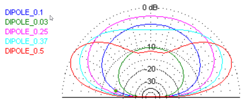
*Figure 3. Dipole radiation patterns vs. height (wavelengths)*

The gain and radiation pattern varies with the height above ground. Heights of 0.1 (blue), 0.25 (fuchsia), and 0.375 (turquoise) wavelengths are most suitable, though at the latter the gain straight up is starting to drop as maximum radiation shifts to lower angles. At 0.5 wavelength (red) there is a significant overhead null, while at 0.03 wavelengths (green) the gain is lower due to ground losses.

The gain also depends on the ground conditions. This plot shows gain vs. height for an 80m dipole over 4 types of ground, to give a sense of the variation:

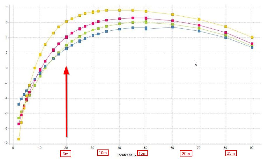
*Figure 4. 80m antenna vertical gain vs. height*

Notice that the peak of the gain curves are very broad, somewhere between 0.13 wavelengths (10m, 35 feet) and 0.25 wavelengths (20m, 65 feet) depending on soil characteristics. However, for any of the soil conditions, a dipole at 0.07 wavelengths (6m or 20 feet), as shown by the red arrow, is within about 3 dB of the peak, and, especially for portable operation, this may be more practical height. (This is also an effective height for 60m and 40m.) With an inverted vee, try to keep the ends at least half that height above the ground. At lower heights, ground losses increase, although contacts are often still possible with the antenna 1m (3 feet) above the ground, or even less.

My recommendation for a maximum height for an NVIS antenna is about 0.3 wavelengths. So, for 80m this would be 24 m (80 feet: conveniently, in Imperial units the maximum height in feet is equal to the wavelength in meters.) At this height, overhead gain is down about 1 dB from the maximum. As shown by the 0.375 wavelength height plot in Figure 3, antennas at greater heights may still work, especially when a lower angle is required, but interference from more distant sources may become more of a problem.

Radiation Angle vs. Height

Radiation straight up isn’t always the optimum direction for somewhat longer paths that are sometimes encountered in what are thought to be NVIS conditions. The following table shows the vertical of maximum radiation for a horizontal dipole at different heights above ground, as well as the 3 dB vertical beamwidth. An “optimized” antenna may trade gain at short distances for a stronger signal at more distant stations with whom they plan to communicate, based on Table 1.

antenna height (wavelengths)	vertical angle of maximum radiation (degrees)	3 dB range of vertical angles (degrees)
0.1	90	38 – 90
0.15	90	34 – 90
0.2	90	30 – 90
0.25	60	24 – 90
0.3	47	21 – 90
0.35	40	18 – 90
0.4	34	16 – 62
0.45	30	14 – 52
0.5	28	13 – 46

Table 2. Typical vertical radiation angles for horizontal antennas at different heights above ground.

Signal Strengths

Signal strengths should generally be fairly strong when using a suitable band, perhaps S9 + 20 dB or more for a 100W transmitter and an efficient antenna. This generally allows sufficient margin for QRP operation, inefficient antennas, and/or a high receive noise level (but not necessarily all at the same time). In my experience, weak signals are due to either band conditions being marginal, or a station problem of some sort (poor antenna, bad coax, high noise level, etc.) Otherwise, small changes in power or antenna gain (less than 6 dB or so) rarely have much impact on the ability to make contacts: that is mostly determined by the ionospheric conditions.

Choice of Antenna

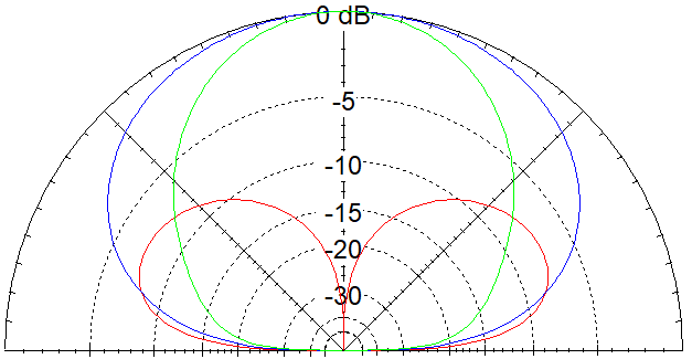
Note that a vertical antenna often has a null straight up, which makes it less effective for paths shorter than about 300km (200 miles) on 80m. The following plot shows the radiation pattern of a vertical (red) compared to a broadside dipole (blue) and a dipole off the ends (green):

*Figure 5. Patterns of vertical (red), dipole broadside (blue) and dipole endwise (green)*

Some of the simplest antennas, like the half wave dipole or inverted vee, and full wavelength loops (either horizontal, or fed for horizontal polarization) work very well for this purpose when they aren’t too high above ground. If you don’t have enough distance available, loading coils or folding the antenna can make it fit. For very limited space applications, a Small Transmitting Loop (mounted in the vertical plane) can also work well, as long as it is reasonably efficient (which is more difficult on 80m and 160m).

The following plot shows the expected relative signal strength for a half-wave dipole for 80m at a height of 10m ( 30 feet ), overlayed on a map centered on the city of St. Louis, Missouri, USA. The contour lines are at intervals of 3 dB, referenced to the maximum value (at very short distances), and are shown for both F-layer and E-layer reflections. The map radius is 800 km (500 miles). The red line in the center of the plot shows the antenna orientation. On 80m, the -3 dB contour is about the same for both E- and F-layer reflections, and at shorter distances propagation will generally be via the F-layer, so E-layer contours are not shown. (Note that these contours do include the effect of signal absorption in the D-layer of the ionosphere, which will reduce signal strength at lower angles of radiation by varying amounts.)

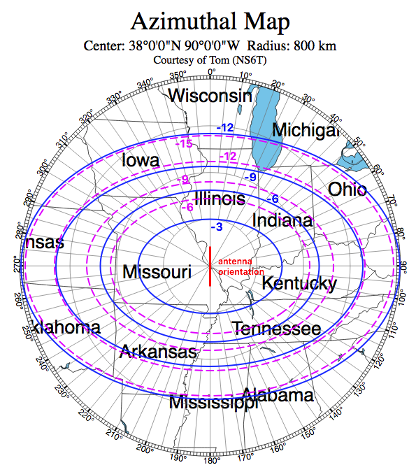
Figure 6. Relative signal strength vs. distance and direction for a half-wave 80m dipole at a height of 10m (30 feet), with contour lines at 3 dB intervals overlayed on a map. Solid blue lines are for F-layer reflections, and dashed purple lines are for E-layer reflections.

Readers wishing to plot this for their own QTH may print out a suitable map from NS6T centered on their location with 800 km radius, and rotate the contour lines shown above to match the orientation of their antenna.

Multiband Operation

Maintaining an appropriate pattern from a single antenna on multiple bands, however, isn’t always an easy task, especially over a 4 : 1 range from 160m through 40m. For example, an OCFD or end-fed half-wave horizontal wire for 80m will have an overhead null in the pattern on the second harmonic on shorter paths:

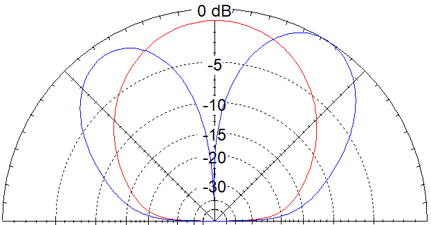
*Figure 7. OCFD patterns on 80m fundamental (red) and 40m 2nd harmonic (blue)*

(But note that lobe at around 60 degrees can be quite effective at distances around 150 to 400 km (95 to 250 miles) off the end of the wire. Horizontal full wave loops tend to have the same problem, though the null might not be as significant for some triangular shapes as it is for squares.

An easy solution is to use multiple dipoles on a common feedpoint for the desired bands, such as my portable dipole kit. This can be simplified, with some savings of space, by using a single loaded element for 40m and 160m that is about the same length as the 80m dipole, although it narrows the operating bandwidth somewhat, and the recommended minimum height for 160m is near the maximum for 40m, so it isn’t perfect. A link dipole can be switched in the field to cover any desired band. The Bow Tie Loop was designed to provide dual-band operation on 160m/80m, and the performance on 40m is often adequate. (Of course, it can also be built for 80m/40m.) An 80m doublet will have added overhead gain on 40m, but a the pattern of a 160m doublet has an overhead null on 40m unless the wires are bent. OCFD antennas will often work well enough on the second harmonic if the antenna is bent 90 degrees at the feedpoint, though it may shift the SWR curve somewhat.

For those using an end-fed wire with a remote tuner, I have a separate article on NVIS designs.

Further NVIS discussions:

What about the US Military AS-2259 NVIS Antenna?
Does lowering the antenna reduce interference?
Can I use a single wire fed against ground with a remote tuner?
What if I want more gain than just a dipole?

Links / References

Elevation Angles and Optimum Antenna Height for Horizontal Dipole Antennas, also available here, is an excellent analysis with measurements of the actual angles of arrival of signals. One important observation is that, in some circumstances, propagation for some paths on 80m and 160m may be via the E layer rather than the F layer, which would require lower angles of radiation. This needs further study.

BACK TO:

antennas for different applications

antennas for Field Day

Beginner’s Corner

Practical Antennas